Draft Climate service for Ostreopsis cf ovata

Time period

1999-2017 (present)

2041-2060 (mid-century, pessimistic scenario)

2081-2100 (end century, pessimistic scenario)

difference : present - mid century

difference : present - end century

Log-10 scale

Date

Drag slider to show a time of the year on the map. Click the play icon to automatically scroll through time.

Scroll or pinch to zoom. Shift-drag to select a region and zoom on it.

Contributors

Main author: S Fabri-Ruiz (LOV, SU-CNRS)
Supervisors: J-O Irisson, R Lemée (LOV, SU-CNRS)
Climate models: S Somot, F Sevault (CNRM, Météo-France); C Ulses, C Estournel, P Marsaleix (LA/LEGOS, OMP)
Ostreopsis data collection: R Lemée, K Drouet (LOV, SU-CNRS); E Berdalet, M Vila, L Viure, (ICM, CSIC); et al

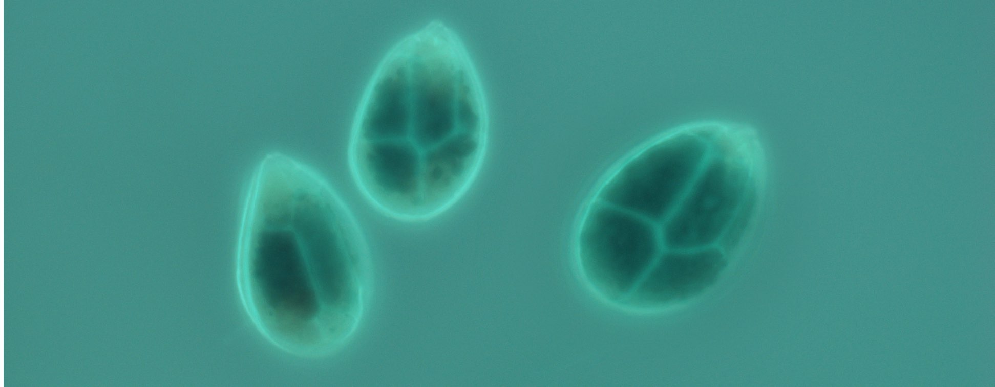
Photo of O. cf ovata, K Drouet

Institutional support

CoCliME for funding and scientific environment

SOMLIT for in situ hydrological data
Copernicus (CMEMS) for present-time physical and biogeochemical reanalyses
Med-CORDEX for climate runs coordination and distribution (CNRM-RCSM4 model)
EUSeaMap for sea bed habitat type
IMEV for hosting this visualisation application

Methods summary

See paper to come

Pixels corresponding to rocky shores or P oceanica beds in the western Mediterranean Bassin (line) were retained based on regional maps. Variables from regional reanalyses of physical and biogeochemical variables were corrected through robust regression to fit in situ data. Climate model runs for the historical period and RCP8.5 emissions scenario (CNRM-RCSM4 for physics, Eco3M-S for biogeochemistry) were also corrected to match the corrected reanalyses in the present time, by matching their cumulative distribution functions (CDF-t); the same correction was then applied to the future time periods. Ostreopsis cf ovata benthic densities were collected over three time series in the North Western Mediterranean. Densities were regressed on physical and biogeochemical variables from the corrected climatic runs through Boosted Regression Trees. The model then allowed to predict the density according to the environmental conditions over the retained pixels for the present time and the two future periods. The average of predicted densities or of their difference among time periods are then represented on a map here.
All analyses were performed in R 3.6.1, with packages tidyverse for data handling and visualisation, gbm for boosted regression. The interactive map is made thanks to leaflet.js with tiles from mapbox.